Benford’s Law: The First-Digit Pattern That Catches Fraud

Benford’s Law Explained: The Mathematical Pattern Hidden in Everyday Numbers

In 1881, a Canadian astronomer named Simon Newcomb noticed something odd about his logarithm books: the pages at the front were noticeably more worn than the ones at the back. The early pages covered numbers starting with 1, 2, and 3. The later pages covered 7, 8, and 9. His colleagues, apparently, were looking up small-digit numbers far more often – and not by accident.

Newcomb published a short paper on it. Almost nobody read it. Fifty-seven years later, a physicist at General Electric named Frank Benford independently found the same pattern, tested it against 20,229 data points pulled from river areas, atomic weights, street addresses, Reader’s Digest articles, and baseball statistics, and published his results in a 1938 paper called “The Law of Anomalous Numbers.” The phenomenon has carried his name ever since – which is itself a bit ironic, since Newcomb got there first.

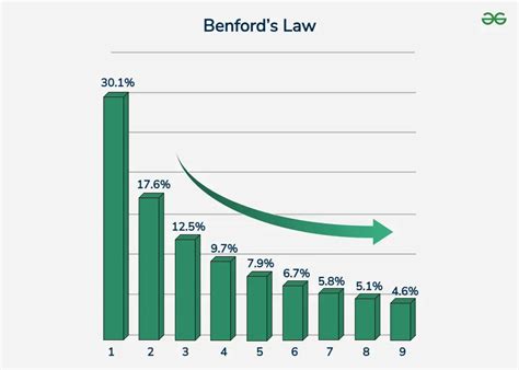
The pattern is this: in many large collections of naturally occurring numbers, the digit 1 appears as the first digit about 30% of the time. The digit 9 appears less than 5% of the time. If digits were evenly distributed, each would show up roughly 11% of the time. They aren’t. The full distribution looks like this:

• 1 → 30.1%
• 2 → 17.6%
• 3 → 12.5%
• 4 → 9.7%
• 5 → 7.9%
• 6 → 6.7%
• 7 → 5.8%
• 8 → 5.1%
• 9 → 4.6%

That slope – steep at 1, nearly flat by 9 – is Benford’s Law. It’s also called the First Digit Law, the Law of Anomalous Numbers, and (rarely) the Newcomb–Benford Law.

Why Does This Happen?

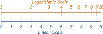
The most useful explanation involves logarithms, though you don’t need to love math for it to make sense. Plot numbers on a logarithmic scale instead of a linear one, and you’ll notice that the distance between 1 and 2 is much larger than the distance between 8 and 9. If you pick random positions on a log scale – which is roughly what naturally occurring data does – you’ll land in the “1 territory” far more often than the “9 territory.”

There’s also a property called scale invariance. Measure a set of rivers in kilometers, then convert to miles. The first-digit distribution of both datasets will be identical. That’s not a coincidence – it’s a mathematical consequence of how logarithms behave under multiplication. Any scale transformation just slides the data along the log axis; it doesn’t change which digits come out on top.

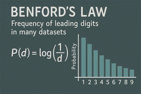
Formally, the probability that the first digit is d (where d goes from 1 to 9) is:

P(d) = log₁₀(1 + 1/d)

Plug in d = 1 and you get log₁₀(2) ≈ 0.301. Plug in d = 9 and you get log₁₀(10/9) ≈ 0.046. That formula generates the entire table above.

What nobody has fully solved is why so many real-world datasets end up logarithmically distributed in the first place. Mathematician Ted Hill produced what’s considered the most rigorous statistical derivation in a 1996 paper, but his explanation still doesn’t constitute a complete proof of why the law applies where it does. The mathematical community is still waiting on that one.

Where Benford’s Law Actually Shows Up

Benford tested his law against areas of 335 rivers, the population sizes of 3,259 U.S. counties, the addresses of 342 people listed in the front section of a copy of American Men of Science, and more than a dozen other datasets. Nearly all of them fit.

Since then, researchers have confirmed the pattern in stock market prices, electricity bills, earthquake magnitudes, death rates, TikTok like counts, and the numerical values appearing in issues of Scientific American. Fibonacci numbers follow Benford’s Law. So do most power-law distributions, which turn up constantly in nature – city sizes, word frequencies, wealth distributions.

The common thread is range. Data has to span multiple orders of magnitude for the law to apply well. Population figures for U.S. counties range from under 100 to several million – that’s many orders of magnitude, and county populations follow Benford’s Law closely. Human heights range from maybe 140 cm to 220 cm – less than one order of magnitude – and they don’t follow it at all.

Assigned numbers never follow it. Phone numbers, Social Security numbers, ZIP codes, student IDs: these are structured by design, not generated by natural processes. Running a Benford analysis on ZIP codes would tell you nothing useful.

The Fraud Detection Application

Economist Hal Varian proposed in 1972 that Benford’s Law could be used to spot manipulation in socioeconomic data submitted to government planning agencies. The core idea: if someone fabricates a dataset of financial figures, they tend to invent numbers that “look” random to a human eye – which means they overuse middle digits like 4, 5, and 6, and underuse 1. People also tend to round, which creates unnatural spikes at specific digits.

The forensic accounting application got its mainstream moment in a 1999 Journal of Accountancy article by Mark Nigrini. He showed that auditors could compare the leading-digit frequencies of a set of financial transactions to the expected Benford distribution and flag deviations for investigation. One case he documented involved an embezzler who wrote checks to himself just below the $100,000 reporting threshold – consistently in the $99,000s – causing the digit 9 to appear as the leading digit far more often than Benford’s Law predicts.

Benford’s Law analysis is now legally admissible as evidence in federal, state, and local courts in the United States. The forensic accounting community includes it in the Fraud Examiners Manual. Auditors at the IRS and accounting firms routinely apply it as a first-pass screening tool on large transaction datasets.

The practical workflow is straightforward: extract the leading digit from each number in a dataset, count how often each digit (1–9) appears, compare those frequencies to the expected Benford percentages, then measure the deviation using a statistical test. The three most common tests are the chi-square test, Mean Absolute Deviation (MAD), and the Kolmogorov–Smirnov test. Each measures something slightly different; in practice, auditors often run all three.

In Excel, this takes about twenty minutes once you know the formula structure. In R, there’s a dedicated package called benford.analysis that automates the whole thing. Python users can do it with pandas in fewer than thirty lines.

The Election Fraud Question

After disputed elections, Benford’s Law tends to reappear in the news. The 2009 Iranian presidential election was analyzed this way; some researchers argued that the digit distribution of vote totals showed statistical anomalies inconsistent with natural data. A 2021 study of the 1994 Brazilian senate election in the state of Bahia applied a base-change variant of the law and found similar signals – in an election that had long been suspected of manipulation but never substantiated.

The problem is that elections are a genuinely contested case for Benford’s Law, and responsible analysts say so. Vote counts for a given candidate in a given county may not span enough orders of magnitude. If a candidate gets between 3,000 and 12,000 votes in most counties, those numbers all start with 1, 2, 3, 4, or occasionally 5 – meaning the data is structurally biased toward smaller digits regardless of whether any fraud occurred. A Benford deviation in that context could mean fraud, or it could just mean the data has a restricted range.

What that means in practice: a Benford anomaly in election data is a reason to look closer. It is not, by itself, evidence of anything. Several statisticians have written specifically about this, noting that the method has been misapplied to make fraud claims that the underlying math doesn’t support. The 2020 U.S. election generated a wave of such claims – essentially all of which were methodologically flawed.

The Limits of the Law

There’s a short list of conditions a dataset needs to meet before Benford’s Law tells you anything useful:

• The dataset has to be large. There’s no firm cutoff, but smaller datasets produce unreliable digit frequencies just because of sampling noise.
• The values have to span multiple orders of magnitude – ideally covering numbers in the tens, hundreds, thousands, and beyond.
• The numbers have to be measured, not assigned. Naturally generated figures (transaction amounts, population counts, stock prices) qualify. Structured codes (account numbers, employee IDs) don’t.
• There can’t be a hard artificial floor or ceiling that distorts the distribution. Hourly wages with a minimum wage floor, for instance, won’t follow Benford’s Law because the data can’t freely range downward past a certain point.

What I find genuinely surprising about this – and it took a few minutes to sit with – is that the law is practically useless for exactly the kinds of data that seem most “natural” to a non-statistician. Human ages follow a restricted range and don’t obey Benford’s Law. Heights, weights, test scores, commute times: none of them do. The law is most powerful on data that feels impersonal and large-scale, like national financial records or geological measurements.

There’s also a statistical trap on the other end: with very large datasets, even a tiny deviation from Benford’s Law will register as statistically significant under a chi-square test. A company with ten million transactions might show a technically significant p-value even though its digit distribution is essentially normal. This is called the excess power problem, and it’s one of the reasons auditors don’t treat a significant test result as proof of anything – it’s a flag, not a verdict.

How to Run a Basic Benford Analysis

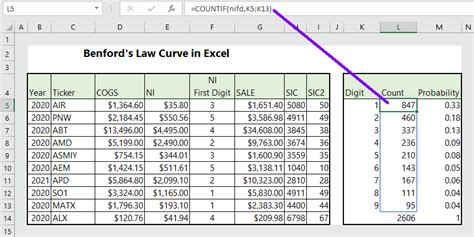
Starting in Excel: suppose you have a column of transaction amounts in column A. In a new column, use =LEFT(TEXT(A2,"0"),1) to extract the leading digit as text. Then use COUNTIF to count how many times each digit (1 through 9) appears. Divide each count by the total number of rows to get observed frequencies. In the next column, enter the expected Benford frequencies (0.301, 0.176, 0.125, etc.). Calculate the absolute difference for each digit and sum them – that gives you the Mean Absolute Deviation, which forensic accountants use as a quick pass/fail metric. A MAD above 0.015 is generally worth investigating; above 0.022 suggests a nonconforming dataset.

In Python:

import pandas as pd
import numpy as np

df = pd.read_csv("transactions.csv")
amounts = df["amount"].dropna()
leading_digits = amounts.astype(str).str.lstrip("0").str[0].astype(int)
observed = leading_digits.value_counts(normalize=True).sort_index()

expected = {d: np.log10(1 + 1/d) for d in range(1, 10)}
expected_series = pd.Series(expected)

mad = (observed - expected_series).abs().mean()
print(f"MAD: {mad:.4f}")

That’s the entire analysis, minus visualization. Add a bar chart comparing observed vs. expected frequencies and you have something an auditor can read.

The R package benford.analysis wraps all of this – digit extraction, chi-square test, MAD, a distortion factor metric, and several diagnostic plots – into a single benford() function call. It’s the fastest path if you’re working in R and want to go from raw data to a professional-grade report.

One thing to check before running any of this: make sure negative numbers and zeros are handled. Leading zeros aren’t digits; negative signs aren’t digits either. Strip them out, or your extraction logic will return garbage. It’s an obvious point, but transaction datasets frequently have both.